Simulation output · 9 scenarios × 12,000 joint paths
Results
Table 1: one-step-ahead forecast accuracy (146-day test window)
| Model | MAE ($) | RMSE ($) |
|---|---|---|
| Seasonal ARIMA(2,1,2)×(1,0,1)₇ | 4,737 | 5,920 |
| LSTM (2 × 48 units) | 4,865 | 6,129 |
The seasonal ARIMA wins on both metrics. Weekly seasonality and payday structure are exactly what a linear seasonal model captures, so its forecast (mean daily redemption ≈ $52,745, forecast cv 0.112) feeds the optimizer.
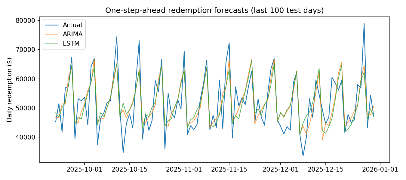
Figure: optimal hedge ratio h* across the 3×3 grid
Monotone in both directions: down each column volatility pulls the hedge up; across each row forecast error pulls it down, all the way to the no-hedge corner where a poor forecast meets a quiet price.
Figure: objective J(h) by volatility (medium demand uncertainty)
Figure: optimizer savings vs. not hedging, % of procurement budget
Up to 12% of the procurement budget at high volatility. The instructive failure is the other direction: a fixed trailing-average rule (h ≈ 0.96 regardless of conditions) happens to sit near the optimum in high-volatility cells but pays up to 0.83% of budget in the regimes where the optimizer says not to hedge, static rules can be accidentally right, but only the optimizer knows when.